Feature Engineering for Ideal Range

A simulation

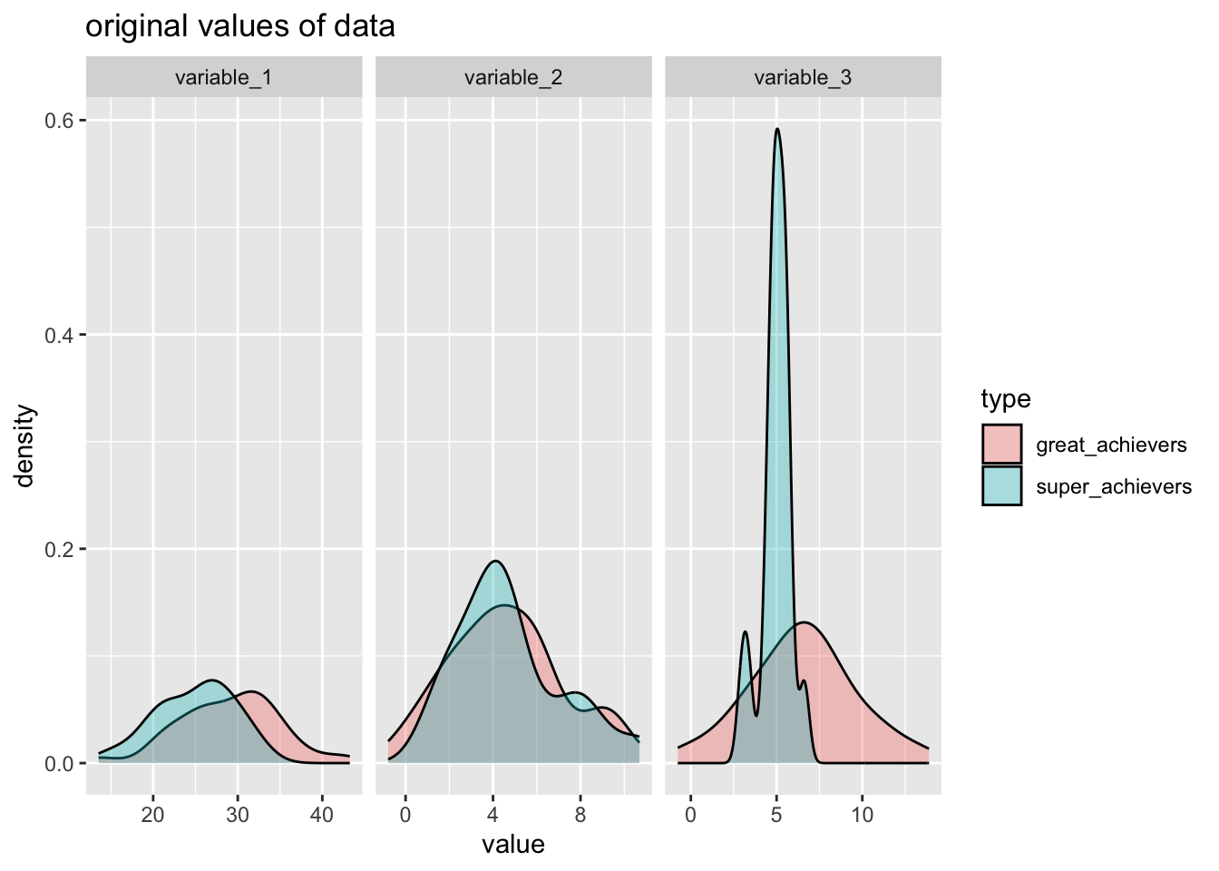
Let’s imagine the group you are interested in (super achievers) score slighly differnt from the (merely) good achievers. In the code below I simulate two groups combine the data and split the data into a training and testset.

We will only look at the testset at the end.

suppressPackageStartupMessages(library(ggplot2))
library(tidyr)
library(recipes)

## Loading required package: dplyr

## 
## Attaching package: 'dplyr'

## The following objects are masked from 'package:stats':
## 
##     filter, lag

## The following objects are masked from 'package:base':
## 
##     intersect, setdiff, setequal, union

## 
## Attaching package: 'recipes'

## The following object is masked from 'package:stats':
## 
##     step

library(rsample)
library(workflows)
library(parsnip)
library(yardstick)

## For binary classification, the first factor level is assumed to be the event.
## Use the argument `event_level = "second"` to alter this as needed.

# simulate super achievers
# wider spread for normal achievers
n = 100
sa_n = ceiling(n/4)
set.seed(1235)

sa <- data.frame(
    type="super_achievers",
    variable_1 = rnorm(sa_n, mean = 25, sd = 5),
    variable_2 = rnorm(sa_n, mean = 4, sd = 2),
    variable_3 = rnorm(sa_n, mean = 5, sd = 1)
)
ga <-data.frame(
    type="great_achievers",
    variable_1 = rnorm(n, mean = 30, sd = 5),
    variable_2 = rnorm(n, mean = 4.5, sd = 3),
    variable_3 = rnorm(n, mean = 6.1, sd = 3)
)
dataset_achievers <- rbind(sa,ga) 
splits<- rsample::initial_split(dataset_achievers, strata=type)

training(splits) %>% 
    pivot_longer(cols = variable_1:variable_3) %>% 
    ggplot(aes(x=value, group=type, fill=type) )+
    geom_density(alpha=1/3)+
    facet_wrap(~name, scales = "free_x") +
    labs(
        title="original values of data"
    )

Different transformations

The (free and internet available) book Feature engineering and selection by Max Kuhn and Kjell Johnson https://bookdown.org/max/FES/ gives awesome advise about feature engineering.

• maybe splines? natural cubic spline
• distance to mean ideal
• sign transformation?

Splines > Spline transformations take a numeric column and create multiple features that, when used in a model, can estimate nonlinear trends between the column and some outcome.

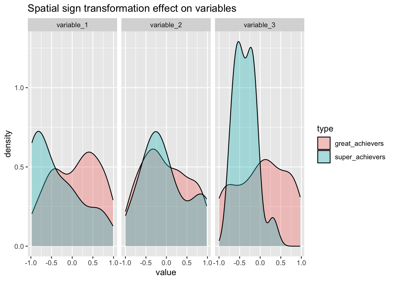
Sign transformation: > This has the effect of making all the samples the same distance from the center of the sphere. (Factors are not allowed.)

I’m using the tidymodels framework to create feature engineering recipes. We prep these recipes on the training data and finally test them out on the testset (that way we don’t leak test information into the trainingset, giving us unfair advantage).

rec_normal<- recipe(training(splits),formula = type~.) %>% 
    step_center(variable_1:variable_3) %>% 
    step_scale(variable_1:variable_3)

rec_normal_int <- rec_normal %>% 
    step_interact(terms= ~variable_1:variable_2) %>% 
    step_interact(terms= ~variable_2:variable_3) %>% 
    step_interact(terms= ~variable_1:variable_3)
rec_sp_sgn <- rec_normal %>% 
    step_spatialsign(variable_1:variable_3)
# splines are hard to explain to stakeholders
# rec_splines<- rec_normal %>% 
#     step_spline_natural(variable_1:variable_3) 

sa_means_sd <- training(splits) %>% 
    filter(type=="super_achievers") %>% 
    summarize(
        m_1 = mean(variable_1),
        m_2 = mean(variable_2),
        m_3 = mean(variable_3),
        sd_1 = sd(variable_1),
        sd_2 = sd(variable_2),
        sd_3 = sd(variable_3)
              )
rec_distance<- recipe(training(splits),formula = type~.) %>% 
    step_mutate(
        distance_var1 = abs(variable_1-sa_means_sd$m_1)/sa_means_sd$sd_1,
        distance_var2 = abs(variable_2-sa_means_sd$m_2)/sa_means_sd$sd_2,
        distance_var3 = abs(variable_3-sa_means_sd$m_3)/sa_means_sd$sd_3,
    ) %>% 
    step_rm(variable_1:variable_3)
rec_distance_sqrt <-recipe(training(splits),formula = type~.) %>% 
    step_mutate(
        distance_var1 = sqrt(abs(variable_1-sa_means_sd$m_1)/sa_means_sd$sd_1),
        distance_var2 = sqrt(abs(variable_2-sa_means_sd$m_2)/sa_means_sd$sd_2),
        distance_var3 = sqrt(abs(variable_3-sa_means_sd$m_3)/sa_means_sd$sd_3),
    ) %>% 
    step_rm(variable_1:variable_3)

rec_distance_sqrt_norm <- rec_distance_sqrt %>% 
    step_BoxCox(distance_var1:distance_var3)

(this doesn’t do anything?)

bake(prep(rec_sp_sgn, training = training(splits)),training(splits)) %>% 
    pivot_longer(cols = variable_1:variable_3) %>% 
    ggplot(aes(x=value, group=type, fill=type) )+
    geom_density(alpha=1/3)+
    facet_wrap(~name, scales = "free_x") +
    labs(
        title="Spatial sign transformation effect on variables"
    )

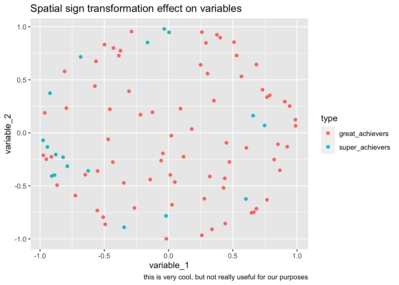
bake(prep(rec_sp_sgn, training = training(splits)),training(splits)) %>%
    ggplot(aes(variable_1, variable_2, color=type))+
    geom_point()+
    labs(
        title="Spatial sign transformation effect on variables",
        caption="this is very cool, but not really useful for our purposes"
    )

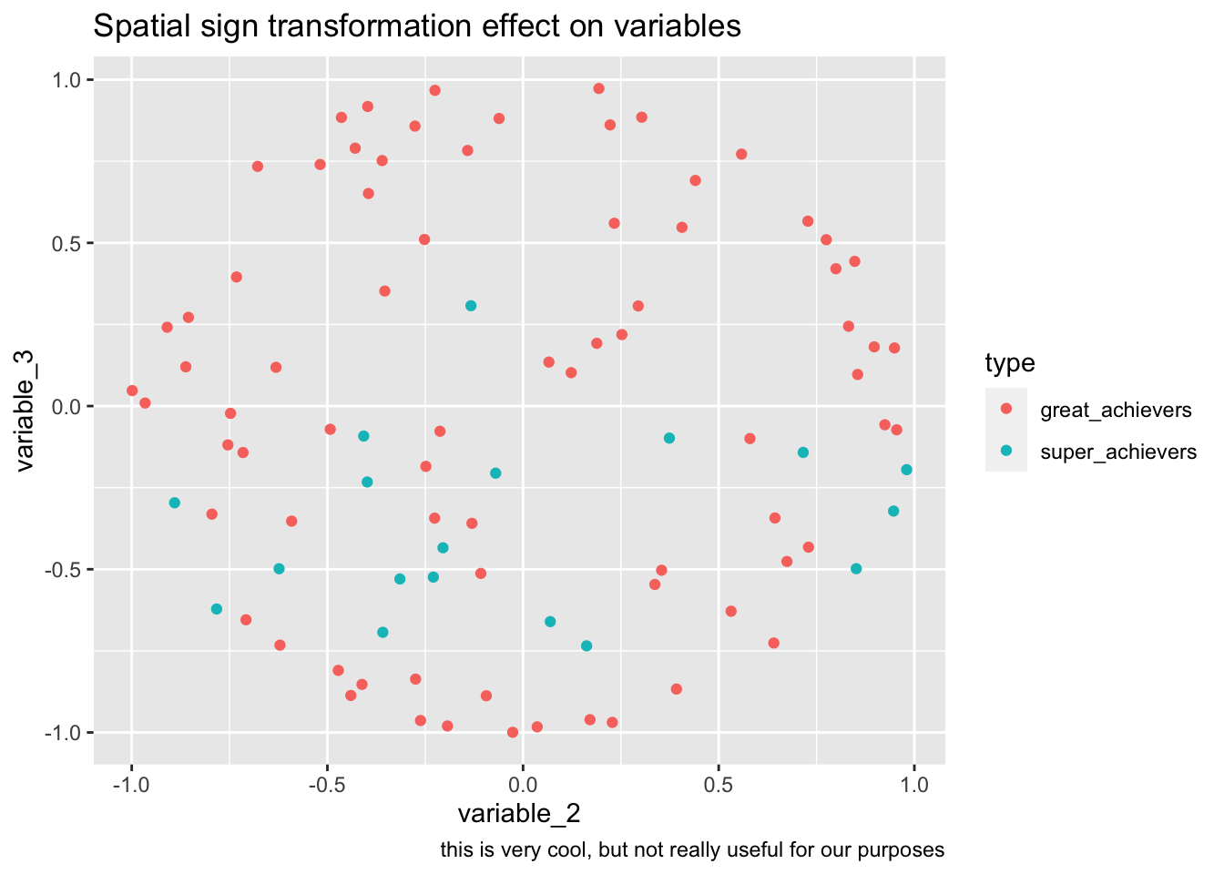
bake(prep(rec_sp_sgn, training = training(splits)),training(splits)) %>%
    ggplot(aes(variable_2, variable_3, color=type))+
    geom_point()+
    labs(
        title="Spatial sign transformation effect on variables",
        caption="this is very cool, but not really useful for our purposes"
    )

(original data is no longer there or course. 93 variables) Splines are fun, but no longer really explainable.

bake(prep(rec_splines, training = training(splits)),training(splits)) %>% 
    pivot_longer(cols = variable_1:variable_3) %>% 
    ggplot(aes(x=value, group=type, fill=type) )+
    geom_density(alpha=1/3)+
    facet_wrap(~name, scales = "free_x") +
    labs(
        title="splines transformation effect on variables"
    )

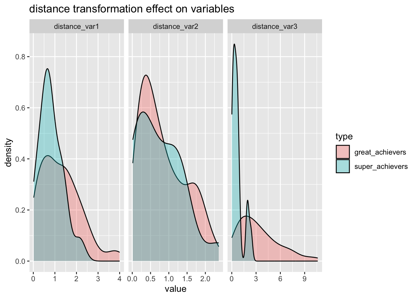
bake(prep(rec_distance, training = training(splits)),training(splits)) %>% 
    pivot_longer(cols = distance_var1:distance_var3) %>% 
    ggplot(aes(x=value, group=type, fill=type) )+
    geom_density(alpha=1/3)+
    facet_wrap(~name, scales = "free_x") +
    labs(
        title="distance transformation effect on variables"
    )

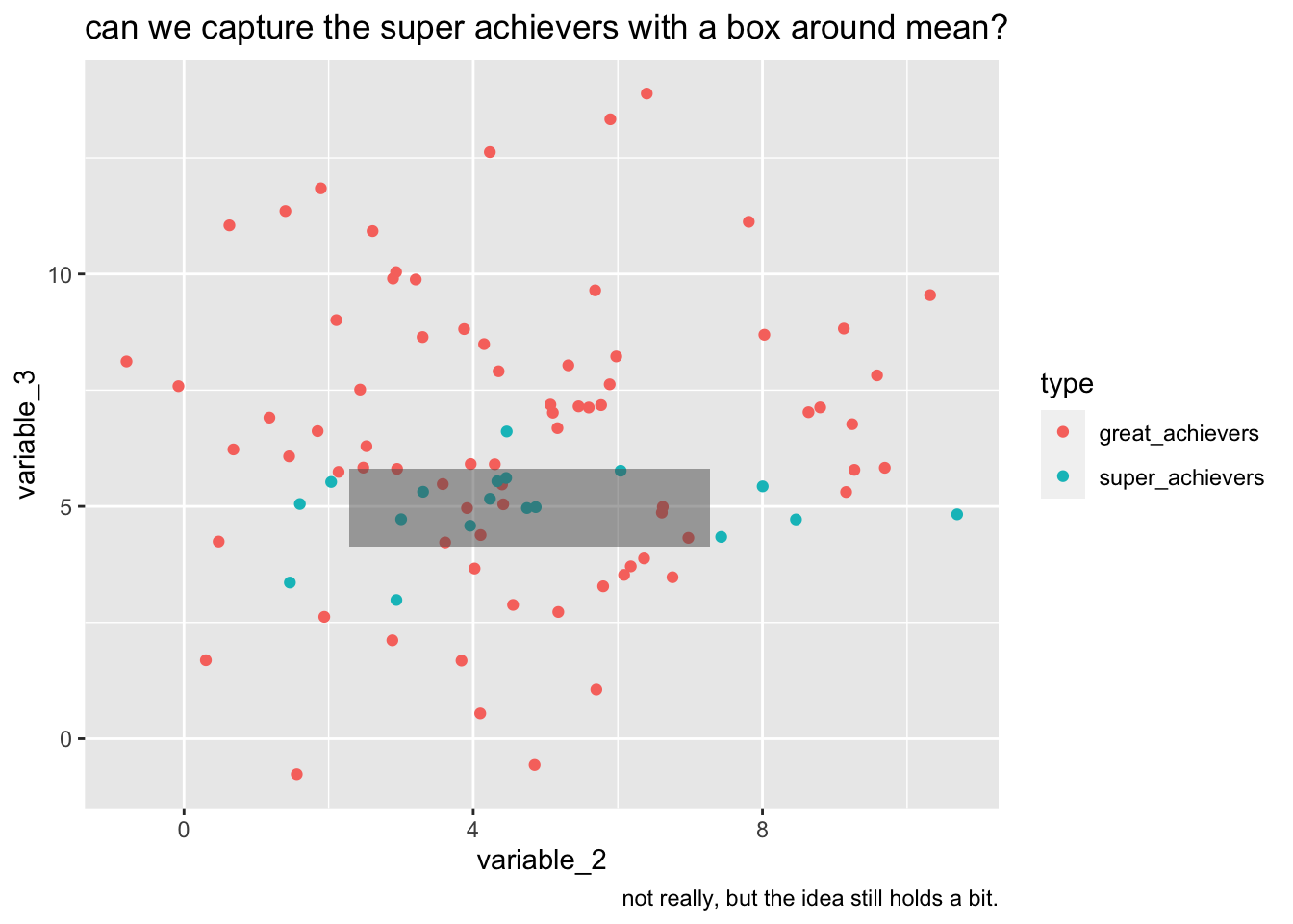
Some more exploration if we can maybe create boundaries.

training(splits) %>% 
    ggplot(aes(variable_2,variable_3, color=type))+
    geom_point()+
    geom_rect(data = sa_means_sd, aes(xmin=m_2-sd_2, xmax=m_2+sd_2, ymin=m_3-sd_3, ymax=m_3+sd_3), inherit.aes=FALSE, alpha=1/2)+
    labs(
        title="can we capture the super achievers with a box around mean?",
        caption="not really, but the idea still holds a bit."
    )

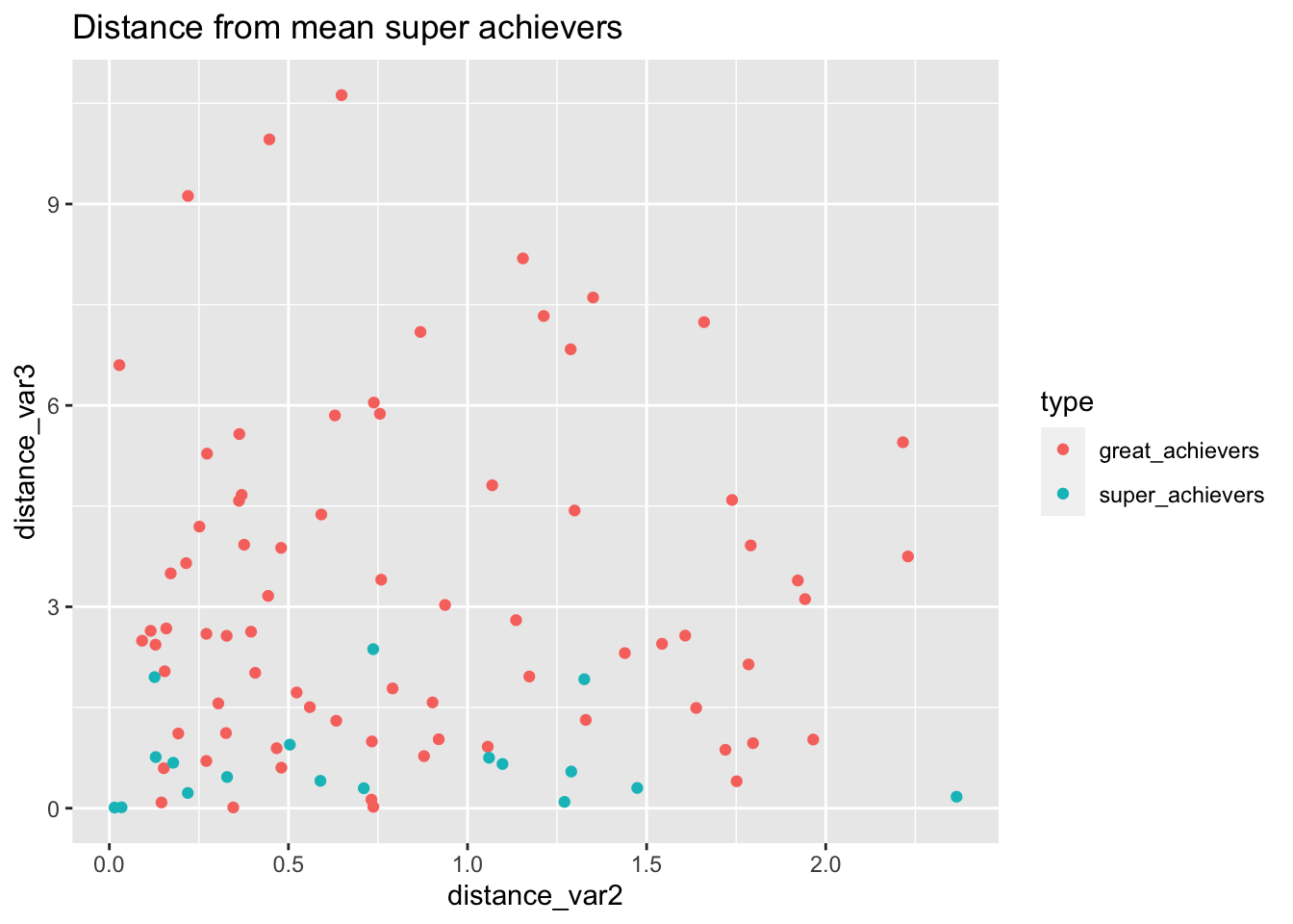
bake(prep(rec_distance, training = training(splits)),training(splits)) %>% 
    ggplot(aes(distance_var2, distance_var3, color=type))+
    geom_point() +
    labs(
        title="Distance from mean super achievers"
    )

bake(prep(rec_distance, training = training(splits)),training(splits)) %>% 
    ggplot(aes(distance_var1, distance_var3, color=type))+
    geom_point() +
    labs(
        title="Distance from mean super achievers"
    )

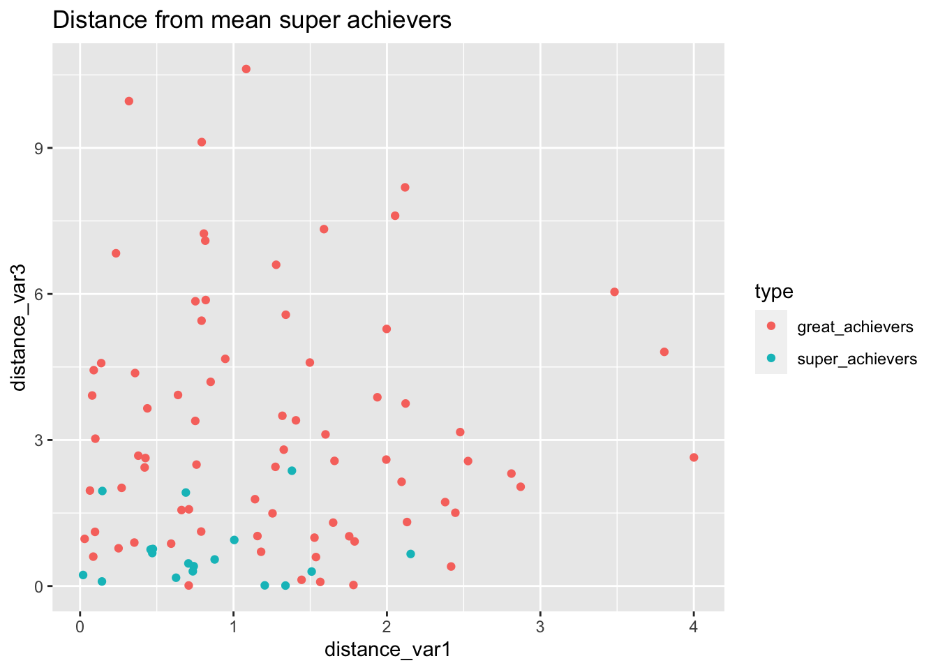
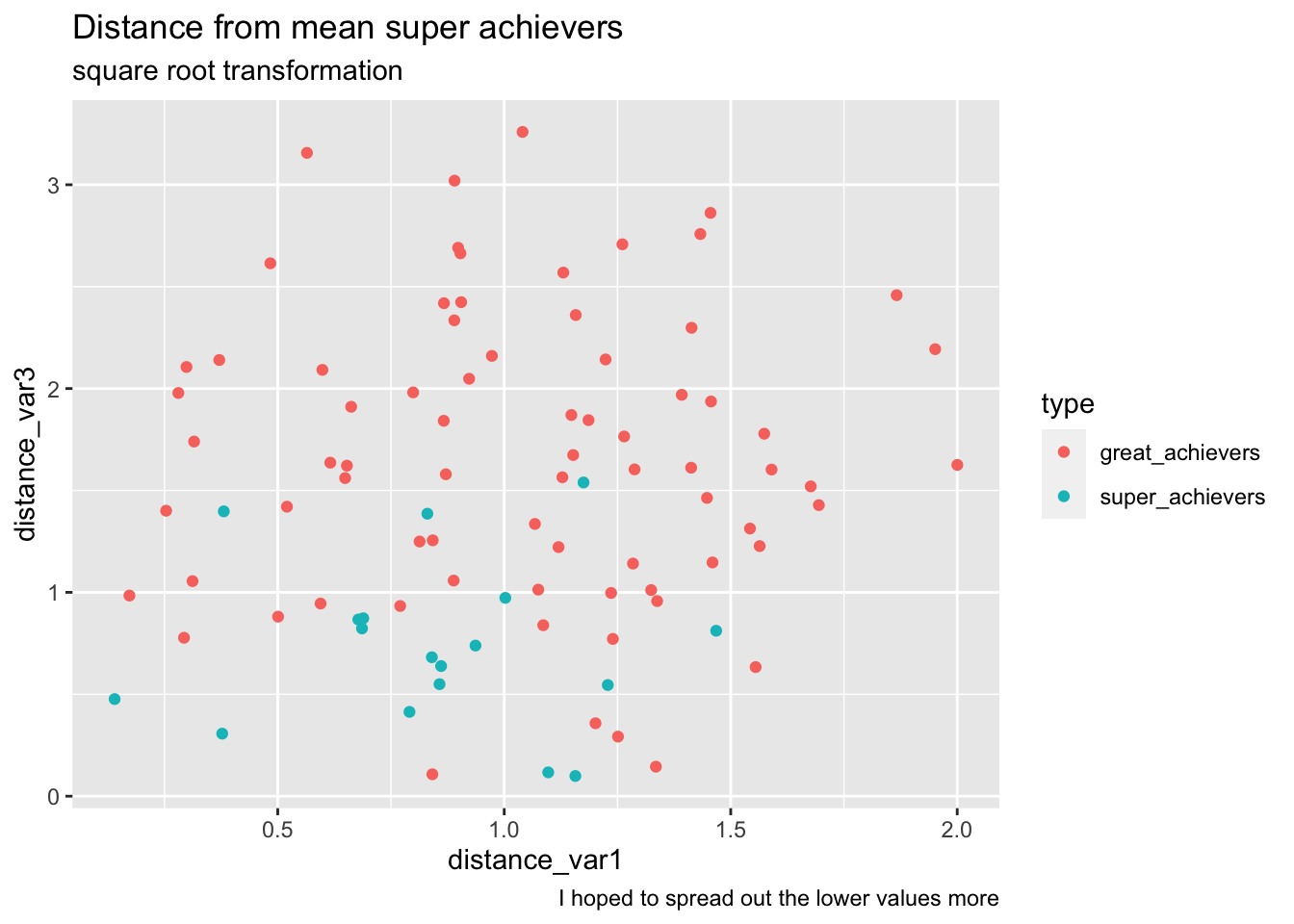
What if we transform the data in a way that spreads out points in the middle? (since we take the aboslute this works. small values are exaggerated.)

bake(prep(rec_distance_sqrt, training = training(splits)),training(splits)) %>% 
    ggplot(aes(distance_var1, distance_var3, color=type))+
    geom_point() +
    labs(
        title="Distance from mean super achievers",
        subtitle="square root transformation",
        caption="I hoped to spread out the lower values more"
    )

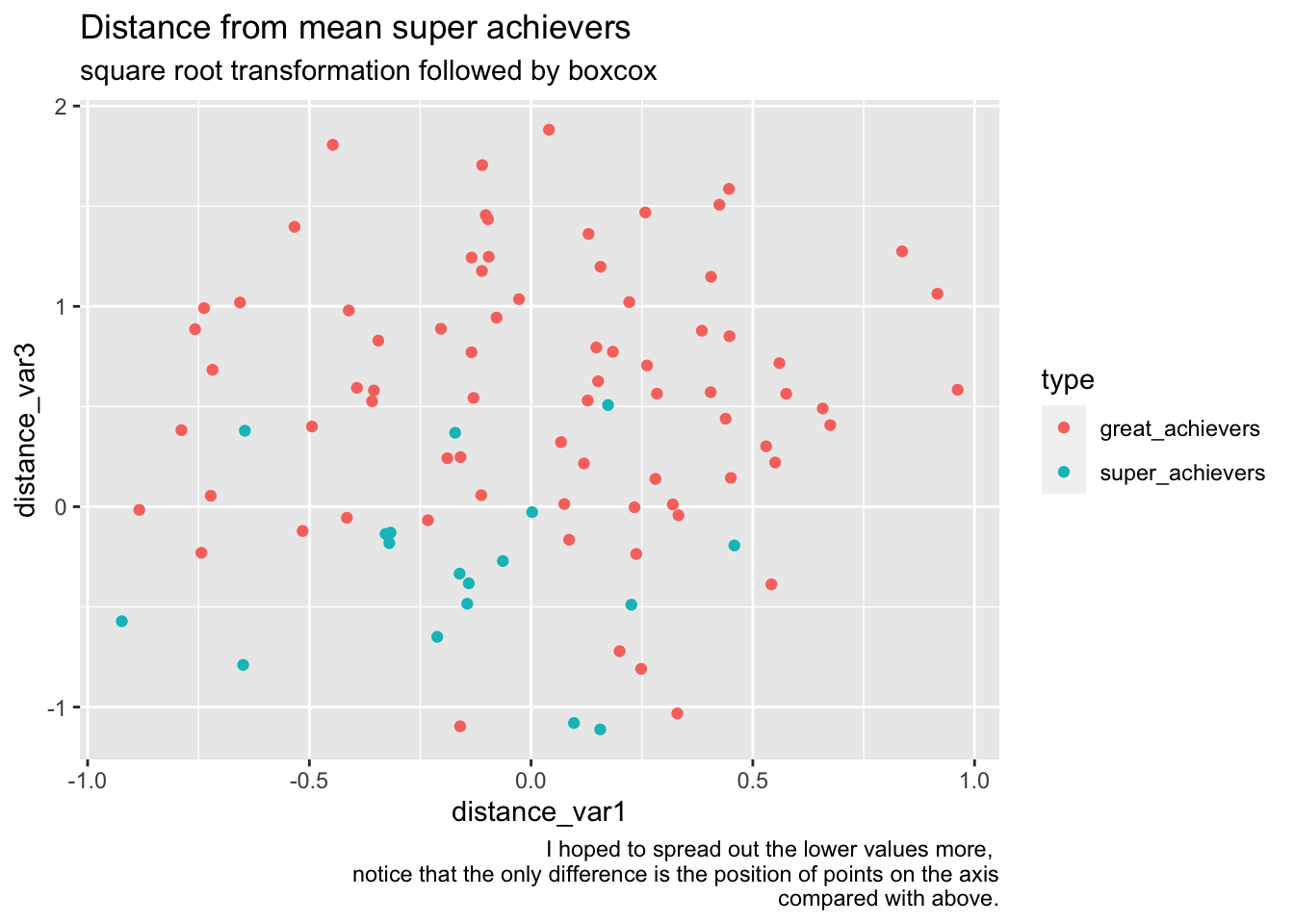
bake(prep(rec_distance_sqrt_norm, training = training(splits)),training(splits)) %>% 
    ggplot(aes(distance_var1, distance_var3, color=type))+
    geom_point() +
    labs(
        title="Distance from mean super achievers",
        subtitle="square root transformation followed by boxcox",
        caption="I hoped to spread out the lower values more, \nnotice that the only difference is the position of points on the axis\n compared with above."
    )

create models

base_model <- logistic_reg(engine="glm")
wf_normal <- workflow(rec_normal, base_model) %>% fit(training(splits))
wf_normal_interact <- workflow(rec_normal_int, base_model) %>% fit(training(splits))
wf_dist <- workflow(rec_distance, base_model) %>% fit(training(splits))
wf_dist_sqrt <- workflow(rec_distance_sqrt, base_model) %>% fit(training(splits))
wf_dist_sqrt_norm <- workflow(rec_distance_sqrt_norm, base_model) %>% fit(training(splits))
#wf_splines <- workflow(rec_splines, base_model) %>% fit(training(splits))
wf_spatsign <- workflow(rec_sp_sgn, base_model) %>% fit(training(splits))

Predict

measures <- yardstick::metric_set(
    bal_accuracy,f_meas,sensitivity, precision
)
# predict with trained workflow
performance_df <- testing(splits) %>% 
    select(type) %>% 
    mutate(
        wf_normal= predict(wf_normal, testing(splits))$.pred_class,
        wf_dist= predict(wf_dist, testing(splits))$.pred_class,
        wf_dist_sqrt=predict(wf_dist_sqrt, testing(splits))$.pred_class,
        wf_dist_sqrt_norm = predict(wf_dist_sqrt_norm, testing(splits))$.pred_class,
        wf_spatsign= predict(wf_spatsign, testing(splits))$.pred_class,
        wf_normal_interact= predict(wf_normal_interact, testing(splits))$.pred_class
        ) %>% 
    # pull the predictions together
    pivot_longer(-type) %>% 
    group_by(name) %>% 
    measures(truth= as.factor(type),estimate=value)

performance_df %>% 
    ggplot(aes(.estimate, name))+
    geom_point()+
    facet_wrap(~.metric,scales = "free_x")+
    labs(
        title="effect of feature engineering",
        caption="notice that the three variants of distance perform the same"
            )

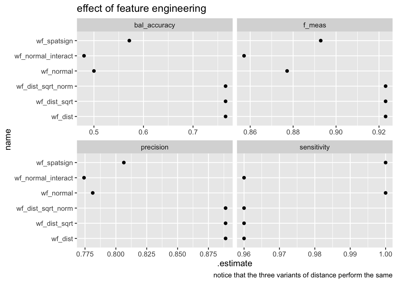
• Sensitivity (true positive rate) is the probability of a positive test result, conditioned on the individual truly being positive.
• F1 score is the harmonic mean of precision and sensitivity