This is a small exploration and best practices for reading data from disk.
One thing is for certain: base R reading and writing to disk are not optimal. However if your data is smallish (~ 5000 rows) the speeds don’t really matter that much. If you only need to load data once, convenience often triumphs speed.
If speed begins to matter, you have multiple options. In base there are
options like read.csv load readRDS. Or you could use another
package. There is data.table, readr, fst or the crosslanguage package
feather. Alternatively there are 2 embedded databases that you could
use, although reading an entire table sort of defeats the purpose of a
database.
In this overview I will show the read performance of
- utils::read.csv
- base::readRDS
- base::read.csv
- base::load
- data.table::fread
- feather::read_feather
- readr::read_csv
- readr::readRDS (wrapper around readRDS but with uncompressed file)
- fst::read.fst
- reading a table from SQLite
- reading a table from MonetDBlite
Apart from this benchmark of an entire dataset, there are other considerations for efficiency in your work. If you only need a few columns or rows from a dataset the databases and fst are excellent choices: they enable you to read in only a selection of columns and rows, without reading in the complete file first. If you do aggregations with window functions the two databases are excellent choices.
Preperation
First we create the dataset
set.seed(23455)
testdataset <-
  data.frame(replicate(10, sample(0:2000, 15 * 10^5, rep = TRUE)),
                 replicate(10, stringi::stri_rand_strings(1000, 5)))
colnames(testdataset) <- tolower(gsub(pattern = "\\.",replacement = "_",colnames(testdataset)))# monetdb doesn't accept special characters or upper case without special treamtent.
and set the datapaths
# fs is a better worked out package to work with files.
if(!fs::dir_exists("data")){fs::dir_create("data")}
path_csv <- 'data/df.csv'
path_feather <- 'data/df.feather'
path_rdata <- 'data/df.RData'
path_rds <- 'data/df.rds'
path_rds_uncompressed <- 'data/df_uncompressed.rds'
path_fst <- 'data/df.fst'
path_sqlite <- "data/df.sqlite"
path_monetdblite <- "data/monetdb"
and load libraries.
# packages for reading and writing
library(feather)
library(data.table)
library(fst)
library(RSQLite)
library(MonetDBLite)
library(readr)
# packages for file manipulations plotting and benchmark
library(fs)
library(DBI)
library(microbenchmark)
library(ggplot2)
and write the files away
# set up database first
consqlite <- DBI::dbConnect(RSQLite::SQLite(),path_sqlite)
conmonet <- DBI::dbConnect(MonetDBLite::MonetDBLite(),path_monetdblite)
# write the files
DBI::dbWriteTable(consqlite,"sqlitedump",testdataset, overwrite = TRUE)
DBI::dbWriteTable(conmonet, "monetdbdump",testdataset, overwrite = TRUE)
#write.csv(testdataset, file = path_csv, row.names = F) # this is too slow, so
write_csv(testdataset, path_csv)
write_feather(testdataset, path_feather)
save(testdataset, file = path_rdata)
saveRDS(testdataset, path_rds)
readr::write_rds(testdataset, path_rds_uncompressed)
write.fst(testdataset, path_fst)
File sizes of saved files
While disk space is usually cheap, sometimes sizes matter. The saveRDS function uses compression by default. FST has a percentage compression you can set and is by default 50.
files <- list.files("data",full.names = TRUE)
info <- file.info(files)
info$size_mb <- info$size/(1024 * 1024)
print(subset(info, select=c("size_mb")),digits = 2)
##                            size_mb
## data/df_uncompressed.rds 114.56589
## data/df.csv              149.42059
## data/df.feather          114.52881
## data/df.fst               34.34178
## data/df.RData             28.54956
## data/df.rds               28.54952
## data/df.sqlite           139.87109
## data/monetdb               0.00015
# sum(fs::dir_info("data/monetdb/")$size) 1.72 kb
Benchmark reading times
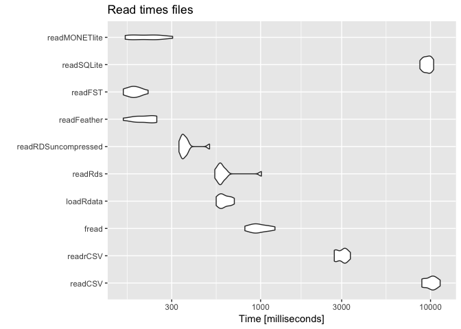
Reading the same file 10 times. Do realise that for the databases this is the worst possible usecase: the database is meant to give you back a subset or calculate and give you the results.
suppressMessages({ # readr is too chatty for this overview
  benchmark <- microbenchmark(
  readCSV = utils::read.csv(path_csv),
  readrCSV = readr::read_csv(path_csv, progress = F),
  fread = data.table::fread(path_csv, showProgress = F),
  loadRdata = base::load(path_rdata),
  readRds = base::readRDS(path_rds),
  readRDSuncompressed = readr::read_rds(path_rds_uncompressed),
  readFeather = feather::read_feather(path_feather),
  readFST = fst::read.fst(path_fst),
  readSQLite = DBI::dbReadTable(consqlite, "sqlitedump"),
  readMONETlite = DBI::dbReadTable(conmonet, "monetdbdump"),
  times = 10)
})

print(benchmark, signif = 2)
## Unit: milliseconds
##                 expr  min   lq  mean median    uq   max neval
##              readCSV 8900 9200 10000  10000 11000 11000    10
##             readrCSV 2700 2800  3000   3100  3200  3400    10
##                fread  810  910   980    960  1100  1200    10
##            loadRdata  550  580   610    600   660   700    10
##              readRds  540  570   620    580   610  1000    10
##  readRDSuncompressed  330  340   370    350   370   500    10
##          readFeather  160  180   210    210   240   250    10
##              readFST  160  170   180    180   200   220    10
##           readSQLite 8700 9000  9600   9600 10000 10000    10
##        readMONETlite  160  170   220    210   250   300    10
Visualize results:

Recommondations for reading files
The recommodations for reading files, on this moment 2019-03-13 , are thus: If you are only using R, don’t write and read CSV. If you must use CSV and you are working with data.table use fread.
FST, Feather, readRDS (use without compression), loadRdata are all useful.
When to use a database?
If you take slices of data a database is almost always the better choice. SQLite and Monetdblite (probably others as well, but I really don’t want to start a db war here) are great choices for a data backend on disk. Monetdb has limitations on the column names, but is extremely fast in aggregations and according to many benchmarks (they really love benchmarking) monetdblite is much faster than sqlite. It all depends on what you want to do with the data. If you have a shiny app where you want to show subsets of data generate queries from the app to an embedded database.
Benchmark for writing files
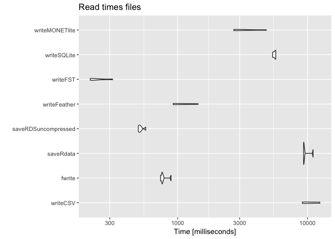
I only did 5 repetitions for this one, because, boy, this is slow!
suppressMessages({ # readr is too chatty for this overview
  benchmark_write <- microbenchmark(
  #writeCSV = utils::write.csv(testdataset,path_csv),
  writeCSV = readr::write_csv(testdataset,path_csv),
  fwrite = data.table::fwrite(testdataset, path_csv),
  saveRdata = base::save(testdataset,file = path_rdata),
  #saveRds = base::saveRDS(testdataset, path_rds),
  saveRDSuncompressed = readr::write_rds(testdataset, path_rds_uncompressed),
  writeFeather = feather::write_feather(testdataset,path_feather),
  writeFST = fst::write.fst(testdataset, path_fst),
  writeSQLite = DBI::dbWriteTable(consqlite,"sqlitedump",testdataset, overwrite = TRUE),
  writeMONETlite = DBI::dbWriteTable(conmonet, "monetdbdump",testdataset, overwrite = TRUE),
  times = 5)
})

print(benchmark_write, signif = 2)
## Unit: milliseconds
##                 expr  min   lq  mean median    uq   max neval
##             writeCSV 9100 9700 11000  10000 12000 12000     5
##               fwrite  740  760   780    760   770   890     5
##            saveRdata 9300 9300  9700   9400  9500 11000     5
##  saveRDSuncompressed  500  500   520    510   520   570     5
##         writeFeather  920  930  1100    970  1200  1400!5
##             writeFST  210  220   250    220   260   320     5
##          writeSQLite 5400 5500  5600   5700  5700  5700     5
##       writeMONETlite 2700 2900  3400   3000  3700  4800     5
Note that for databases there is often a highly optimized csv reader
Visualize results:

Recommondations for writing files
MonetDBLite::monetdblite_shutdown()
DBI::dbDisconnect(consqlite)
fs::dir_delete("data")
Versions are important here. My machine was like this:
sessioninfo::session_info()
## ─ Session info ──────────────────────────────────────────────────────────
##  setting  value
##  version  R version 3.5.1 (2018-07-02)
##  os       macOS  10.14.3
##  system   x86_64, darwin18.2.0
##  ui       X11
##  language (EN)
##  collate  en_US.UTF-8
##  ctype    en_US.UTF-8
##  tz       Europe/Amsterdam
##  date     2019-03-12
##
## ─ Packages ──────────────────────────────────────────────────────────────
##  package        * version    date       lib
##  assertthat       0.2.0      2017-04-11 [2]
##  bit              1.1-14     2018-05-29 [1]
##  bit64            0.9-7      2017-05-08 [1]
##  blob             1.1.1      2018-03-25 [1]
##  cli              1.0.1      2018-09-25 [2]
##  codetools        0.2-16     2018-12-24 [3]
##  colorspace       1.4-0      2019-01-13 [1]
##  crayon           1.3.4      2017-09-16 [2]
##  data.table     * 1.12.1     2019-03-08 [1]
##  DBI            * 1.0.0.9001 2019-01-29 [1]
##  digest           0.6.18     2018-10-10 [2]
##  dplyr            0.8.0.1    2019-02-15 [1]
##  evaluate         0.13       2019-02-12 [1]
##  feather        * 0.3.2      2019-01-07 [1]
##  fs             * 1.2.6      2018-08-23 [2]
##  fst            * 0.8.10     2018-12-14 [1]
##  ggplot2        * 3.1.0      2018-10-25 [2]
##  glue             1.3.0      2018-07-17 [2]
##  gtable           0.2.0      2016-02-26 [2]
##  hms              0.4.2      2018-03-10 [2]
##  htmltools        0.3.6      2017-04-28 [2]
##  knitr            1.22       2019-03-08 [1]
##  lazyeval         0.2.1      2017-10-29 [2]
##  magrittr         1.5        2014-11-22 [2]
##  memoise          1.1.0      2017-04-21 [2]
##  microbenchmark * 1.4-6      2018-10-18 [1]
##  MonetDBLite    * 0.6.0      2018-07-27 [1]
##  munsell          0.5.0      2018-06-12 [2]
##  pillar           1.3.1      2018-12-15 [1]
##  pkgconfig        2.0.2      2018-08-16 [2]
##  plyr             1.8.4      2016-06-08 [2]
##  purrr            0.3.1      2019-03-03 [1]
##  R6               2.4.0      2019-02-14 [2]
##  Rcpp             1.0.0      2018-11-07 [2]
##  readr          * 1.3.1      2018-12-21 [1]
##  rlang            0.3.1      2019-01-08 [1]
##  rmarkdown        1.11       2018-12-08 [2]
##  RSQLite        * 2.1.1.9002 2019-01-29 [1]
##  scales           1.0.0      2018-08-09 [2]
##  sessioninfo      1.1.1      2018-11-05 [2]
##  stringi          1.3.1      2019-02-13 [2]
##  stringr          1.4.0      2019-02-10 [1]
##  tibble           2.0.1      2019-01-12 [1]
##  tidyselect       0.2.5      2018-10-11 [2]
##  withr            2.1.2      2018-03-15 [2]
##  xfun             0.5        2019-02-20 [1]
##  yaml             2.2.0      2018-07-25 [2]
##  source
##  CRAN (R 3.5.1)
##  CRAN (R 3.5.1)
##  CRAN (R 3.5.1)
##  CRAN (R 3.5.1)
##  CRAN (R 3.5.1)
##  CRAN (R 3.5.1)
##  CRAN (R 3.5.1)
##  CRAN (R 3.5.1)
##  local
##  Github (r-dbi/DBI@c7333be)
##  CRAN (R 3.5.1)
##  CRAN (R 3.5.1)
##  CRAN (R 3.5.1)
##  CRAN (R 3.5.1)
##  CRAN (R 3.5.1)
##  CRAN (R 3.5.1)
##  CRAN (R 3.5.1)
##  CRAN (R 3.5.1)
##  CRAN (R 3.5.1)
##  CRAN (R 3.5.1)
##  CRAN (R 3.5.1)
##  CRAN (R 3.5.1)
##  CRAN (R 3.5.1)
##  CRAN (R 3.5.1)
##  CRAN (R 3.5.1)
##  CRAN (R 3.5.1)
##  CRAN (R 3.5.1)
##  CRAN (R 3.5.1)
##  CRAN (R 3.5.1)
##  CRAN (R 3.5.1)
##  CRAN (R 3.5.1)
##  CRAN (R 3.5.1)
##  CRAN (R 3.5.1)
##  CRAN (R 3.5.1)
##  CRAN (R 3.5.1)
##  CRAN (R 3.5.1)
##  CRAN (R 3.5.1)
##  Github (rstats-db/RSQLite@c347308)
##  CRAN (R 3.5.1)
##  CRAN (R 3.5.1)
##  CRAN (R 3.5.1)
##  CRAN (R 3.5.1)
##  CRAN (R 3.5.1)
##  CRAN (R 3.5.1)
##  CRAN (R 3.5.1)
##  CRAN (R 3.5.1)
##  CRAN (R 3.5.1)
##
## [1] /Users/roelhogervorst/Library/R/3.x/library
## [2] /usr/local/lib/R/3.5/site-library
## [3] /usr/local/Cellar/r/3.5.1/lib/R/library
Further reading
- https://appsilon.com/fast-data-loading-from-files-to-r/ “From 2017-04-11, used the same data and approach for reading files, but not all of these options”
- https://kbroman.org/blog/2017/04/30/sqlite-feather-and-fst/ “2017-04-30, another comparison between fst, sqlite and feather, also looks into write performance”